Conley Theory

The main motivation for ConleyDynamics.jl is the development of an accessible tool for studying the global dynamics of multivector fields on Lefschetz complexes. Having already discussed the latter, we now turn our attention to multivector fields and their global dynamics. This involves a detailed discussion of multivector fields, isolated invariant sets, their Conley index, as well as Morse decompositions and connection matrices. We also briefly compare the different connection matrix algorithms which are provided by the package. Finally, we address Forman's Morse complex and the functions that can be used to work with it.

Multivector Fields

Suppose that $X$ is a Lefschetz complex as described in Lefschetz Complexes, see in particular the definition in Basic Lefschetz Terminology. Assume further that the Lefschetz complex is defined over a field $F$, which is either the rational numbers $\mathbb{Q}$ or a finite field of prime order. Then a multivector field on $X$ is defined as follows.

Recall from our detailed discussion in Basic Lefschetz Terminology that a set $V \subset X$ is called locally closed if its mouth $\mathrm{mo}\, V = \mathrm{cl}\, V \setminus V$ is closed, where closedness in turn is defined via the face relation in a Lefschetz complex. This implies that for each multivector $V \in \mathcal{V}$ the relative homology $H_*(\mathrm{cl}\, V, \mathrm{mo}\, V)$ is well-defined, and it allows for the following classification of multivectors:

• A critical multivector is a multivector for which $H_*(\mathrm{cl}\, V, \mathrm{mo}\, V) \neq 0$.
• A regular multivector is a multivector for which $H_*(\mathrm{cl}\, V, \mathrm{mo}\, V) = 0$.

Since a multivector is locally closed, it is a Lefschetz subcomplex of $X$ as well, and we have already seen that its Lefschetz homology satisfies $H_*(V) \cong H_*(\mathrm{cl}\, V, \mathrm{mo}\, V)$. For more details, see Relative Homology.

The above classification of multivectors is motivated by the case of classical Forman vector fields. These are a special case of multivector fields, in that they also form a partition of the underlying Lefschetz complex. This time, however, there are only two types of multivectors:

• A critical cell is a multivector consisting of exactly one cell of the Lefschetz complex. One can easily see that in this case the $k$-th homology group is isomorphic to $F$, as long as the cell has dimension $k$. All other homology groups vanish. Thus, every critical cell is a critical multivector.
• A Forman arrow is a multivector consisting of two cells $\sigma^-$ and $\sigma^+$, where $\sigma^-$ is a facet of $\sigma^+$. In other words, one has to have $\kappa(\sigma^+, \sigma^-) \neq 0$, which also implies that $1 + \dim\sigma^- = \dim\sigma^+$. One can show that all homology groups of a Forman arrow are zero, and therefore it is a regular multivector.

In ConleyDynamics.jl, multivector fields can be created in two different ways. The direct method is to specify all multivectors of length larger than one in an array of type Vector{Vector{Int}} or Vector{Vector{String}}, depending on whether the involved cells are referenced via their indices or labels. Recall that it is easy to convert between these two forms using the command convert_cellsubsets. The subsets specified by the vector entries have to be disjoint. They do not, however, have to exhaust the underlying Lefschetz complex $X$. Any cells that are not part of a specified multivector will be considered as one-element critical cells. This reduces the size of the representation in many situations.

For large Lefschetz complexes, the above method becomes quickly impractical. In such a case it is easier to determine a multivector field indirectly, through a mechanism involving dynamical transitions. This is based on the following result.

The above result shows that as long as one has an idea about the transitions that a system has to be allowed to do, one can always find a smallest multivector field which realizes them. Needless to say, if too many transitions are specified, then it is possible that the result leads to the trivial multivector field $\mathcal{V} = \{ X \}$. In most cases, however, the resulting multivector field is more useful. See also the examples later in this section of the manual.

The package ConleyDynamics.jl provides a number of functions for creating and manipulating multivector fields on Lefschetz complexes:

• The function create_mvf_hull implements the above theorem on dynamical transitions. It expects two input arguments: A Lefschetz complex lc, as well as a vector mvfbase that defines the dynamical transitions in $\mathcal{D}$. The latter has to have type Vector{Vector{Int}} or Vector{Vector{String}}.
• The function mvf_forward_orbit determines the forward orbit of a given cell or set of cells, with respect to an underlying multivector field. More precisely, it returns all multivectors that can be reached from the source cells, and critical cells in the forward orbit are included as singletons. This function has four different signatures:
  1. mvf_forward_orbit(lc::LefschetzComplex, mvf::CellSubsets, cs::Cells)
  2. mvf_forward_orbit(lc::LefschetzComplex, mvf::CellSubsets, c::Cell)
  3. mvf_forward_orbit(lc::LefschetzComplex, mvf::CellSubsets, cs::Cells, n::Int)
  4. mvf_forward_orbit(lc::LefschetzComplex, mvf::CellSubsets, c::Cell, n::Int)
  In all cases, the underlying Lefschetz complex is lc, and mvf denotes the multivector field. In the first and third case, cs is a vector of starting cells, while in the second and fourth case the orbit starts only at a single cell c. Finally, the first two methods determine the complete forward orbit, while the last two only consider at most n transitions. While the forward orbit is given as a collection of multivectors, this can easily be converted to a collection of cells using cellsubsets_to_cells.
• The function mvf_backward_orbit determines the backward orbit of a given cell or set of cells, i.e., it finds all cells which are transported in forward time to the given source cells. This function has also four signatures, completely analogous to the previous one.
• The function mvf_neighborhood computes a multivector neighborhood of a cell or set of cells. It returns all multivectors of the given multivector field that form a neighborhood of the given cells with a collar width of n. More precisely, for n = 0 one obtains the multivectors intersecting the cells in sources, while for n >= 1 the function returns all multivectors from level n-1, together with all multivectors whose closure intersects the closure of the level n-1 neighborhood. Critical cells in this neighborhood will be returned as singletons.
• The function mvf_length returns the number of all multivectors of a given multivector field. This not only includes the multivectors explicitly listed in the argument vector mvf, but also the number of all singletons, which are always critical multivectors.
• The function mvf_critical determines all critical multivectors of the specified multivector field. This includes both the implied singletons, as well as the multivectors explicitly listed in the argument vector mvf which have nontrivial homology.
• The function mvf_regular returns all regular multivectors of the specified multivector field, i.e., all multivectors whose homology groups are all trivial.
• The function mvf_information displays basic information about a given multivector field. It expects both a Lefschetz complex and a multivector field as arguments, and returns a Dict{String,Any} with the information. The keys of this dictionary are as follows:
  • "N mv": Number of multivectors
  • "N critical": Number of critcal multivectors
  • "N regular": Number of regular multivectors
  • "Lengths critical": Length distribution of critical multivectors
  • "Lengths regular": Length distribution of regular multivectors
  In the last two cases, the dictionary entries are vectors of pairs (length,frequency), where each pair indicates that there are frequency multivectors of length length.
• mvf_is_acyclic determines whether a multivector field forms an acyclic partition of the underlying Lefschetz complex or not, and returns the corresponding boolean value. If the multivector field is acyclic, then it is gradient-like, otherwise it contains nontrivial recurrent sets.
• The function extract_multivectors expects as input arguments a Lefschetz complex and a multivector field, as well as a list of cells specified as a Vector{Int} or a Vector{String}. It returns a list of all multivectors that contain the specified cells.
• The function create_planar_mvf creates a multivector field which approximates the dynamics of a given planar vector field. It expects as arguments a two-dimensional Lefschetz complex, a vector of planar coordinates for the vertices of the complex, as well as a function which implements the vector field. It returns a multivector field based on the dynamical transitions induced by the vector field directions on the vertices and edges of the Lefschetz complex. While the complex does not have to be a triangulation, it is expected that the one-dimensional cells are straight line segments between the two boundary vertices.
• The utility function planar_nontransverse_edges expects the same arguments as the previous one, and returns a list of nontransverse edges as Vector{Int}, which contains the corresponding edge indices. The optional parameter npts determines how many points along an edge are evaluated for the transversality check.
• The function create_spatial_mvf creates a multivector field which approximates the dynamics of a given spatial vector field. While it expects the same arguments as its planar counterpart, the Lefschetz complex has to be of one of the following two types:
  • The Lefschetz complex is a tetrahedral mesh of a region in three dimensions, i.e., it is a simplicial complex.
  • The Lefschetz complex is a three-dimensional cubical complex, i.e., it is the closure of a collection of three-dimensional cubes in space.
  In the second case, the vertex coordinates can be slightly perturbed from the original position in the cubical lattice, as long as the overall structure of the complex stays intact. In that case, the faces are interpreted as Bezier surfaces with straight edges.

All of these functions will be illustrated in more detail in the examples which are presented later in this section. See also the Tutorial for another planar vector field analysis.

Invariance and Conley Index

A multivector field induces dynamics on the underlying Lefschetz complex through the iteration of a multivalued map. This flow map is given by

\[ \Pi_{\mathcal V}(x) = \mathrm{cl}\, x \cup [x]_{\mathcal V} \qquad\text{ for all }\qquad x \in X\]

where $[x]_{\mathcal V}$ denotes the unique multivector in ${\mathcal V}$ which contains $x$. The definition of the flow map shows that the induced dynamics combines two types of behavior:

• From a cell $x$, it is always possible to flow towards the boundary of the cell, i.e., to any one of its faces.
• In addition, it is always possible to move freely within a multivector.

The multivalued map $\Pi_{\mathcal V} : X \multimap X$ naturally leads to a solution concept for multivector fields. A path is a sequence $x_0, x_1, \ldots, x_n \in X$ such that $x_k \in \Pi_{\mathcal{V}}(x_{k-1})$ for all indices $k = 1,\ldots,n$. Paths of bi-infinite length are called solutions. More precisely, a solution of the combinatorial dynamical system induced by the multivector field is then a map $\rho : \mathbb{Z} \to X$ which satisfies $\rho(k+1) \in \Pi_{\mathcal V}(\rho(k))$ for all $k \in \mathbb{Z}$. We say that this solution passes through the cell $x \in X$ if in addition one has $\rho(0) = x$. It is clear from the definition of the flow map that every constant map is a solution, since we have the inclusion $x \in \Pi_{\mathcal V}(x)$. Thus, rather than considering solutions in the above (classical) sense, we focus on a more restrictive notion.

The notion of essential solution has its origin in the distinction between critical and regular multivectors. In Forman's theory, which is based on classical Morse theory, critical cells correspond to stationary solutions or equilibria of the underlying flow. Thus, it has to be possible to stay in a critical multivector for all times, whether in forward or backward time, or even for all times. On the other hand, a Forman arrow indicates prescribed non-negotiable motion, and therefore a regular multivector corresponds to motion which goes from the multivector to its mouth.

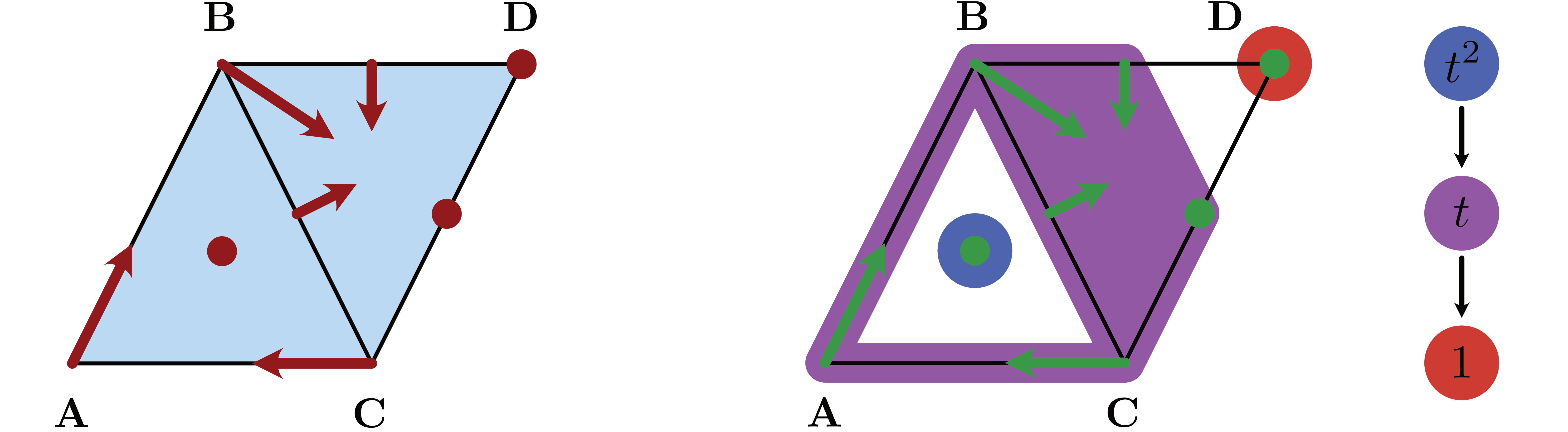
The multivector field from the package logo, which is shown in the accompanying image, consists of three critical cells, two Forman arrows, as well as one multivector which consists of four cells. Beyond the constant essenetial solutions in each of the three critical cells, another essential solution is the periodic orbit

\[ \rho_P \;\text{ given by }\; \ldots \to \mathbf{A} \to \mathbf{AB} \to \mathbf{B} \to \mathbf{BCD} \to \mathbf{C} \to \mathbf{AC} \to \mathbf{A} \to \ldots\]

Notice that this is just one of many realizations of this particular periodic motion, since an essential solution can take many different paths through a multivector.

Using the concept of essential solutions we can now introduce the notion of invariance. Informally, we say that a subset of a Lefschetz complex is invariant if through every cell in the set there exists an essential solution which stays in the set. In other words, we have the choice of staying in the set, even though there might be other solutions that do leave. More generally, for every subset $A \subset X$ one can ask whether there are elements $x \in A$ for which there exists an essential solution which passes through $x$ and stays in $A$ for all times. This leads to the definition of the invariant part of $A$ as

\[ \mathrm{Inv}_{\mathcal{V}}(A) = \left\{ x \in A \, : \, \text{there exists an essential solution } \rho : \mathbb{Z} \to A \text{ through } x \right\}\]

It is certainly possible that the invariant part of a set is empty. If, however, the invariant part of $A$ is all of $A$, i.e., if we have $\mathrm{Inv}_{\mathcal{V}}(A) = A$, then the set $A$ is called invariant. In the context of our above logo example, the image of the essential solution $\rho_P$ is clearly an invariant set.

Invariant sets are the fundamental building blocks for the global dynamics of a dynamical system. Yet, in general they are difficult to study. Conley realized in [Con78] that if one restricts the attention to a more specialized notion of invariance, then topological methods can be used to formulate a coherent general theory. For this, we need to introduce the notion of isolated invariant set:

It is clear that the whole Lefschetz complex $X$ isolates its invariant part. Therefore, the set $\mathrm{Inv}_{\mathcal{V}}(X)$ is an isolated invariant set. Moreover, one can readily show that if $N$ is an isolating set for an isolated invariant set $S$, then any closed set $S \subset M \subset N$ also isolates $S$. Thus, the closure $\mathrm{cl}\, S$ is the smallest isolating set for $S$. With these observations in mind, one obtains the following result from [LKMW23]:

Returning to our earlier logo example, notice that the cells visited by the periodic essential solution $\rho_P$ do not form an isolated invariant set, but rather just an invariant set. However, if we consider the larger set $S_P$ which consists of all cells except for the cells $\mathbf{ABC}$ and $\mathbf{D}$, then we do obtain an isolated invariant set which contains the periodic orbit $\rho_P$.

With this characterization at hand, identifying isolated invariant sets becomes straightforward. In addition, since isolated invariant sets are locally closed, we can now also define their Conley index:

Since the Conley index is nothing more than the relative homology of the closure-mouth-pair associated with a locally closed set, one could easily use the homology functions described in Homology for its computation. However, we have included a wrapper function to keep the notation uniform. In addition, ConleyDynamics.jl contains a function which provides basic information about an isolated invariant set. These two functions can be described as follows:

• The function conley_index determines the Conley index of an isolated invariant set. It expects a Lefschetz complex as its first argument, while the second one has to be a list of cells which specifies the isolated invariant set, and which is either of type Vector{Vector{Int}} or Vector{Vector{String}}. An error is raised if the second argument does not specify a locally closed set.
• The function isoinvset_information expects a Lefschetz complex lc::LefschetzComplex, a multivector field mvf::CellSubsets, as well as an isolated invariant set iis::Cells as its three arguments. It returns a Dict{String,Any} with the information. The keys of this dictionary are as follows:
  • "Conley index" contains the Conley index of the isolated invariant set.
  • "N multivectors" contains the number of multivectors in the isolated invariant set.

Morse Decompositions

We now turn our attention to the global dynamics of a combinatorial dynamical system. This is accomplished through the notion of Morse decomposition, and it requires some auxilliary definitions:

• Suppose we are given a solution $\varphi : \mathbb{Z} \to X$ for the multivector field $\mathcal{V}$. Then the long-term limiting behavior of $\varphi$ can be described using the ultimate backward and forward images

  \[ \mathrm{uim}^- \varphi = \bigcap_{t \in \mathbb{Z}^-} \varphi\left( (-\infty,t] \right) \qquad\text{and}\qquad \mathrm{uim}^+ \varphi = \bigcap_{t \in \mathbb{Z}^+} \varphi\left( [t,+\infty) \right) .\]

  Notice that since $X$ is finite, there has to exist a $k \in \mathbb{N}$ such that

  \[ \mathrm{uim}^- \varphi = \varphi\left( (-\infty,-k] \right) \neq \emptyset \qquad\text{and}\qquad \mathrm{uim}^+ \varphi = \varphi\left( [k,+\infty) \right) \neq \emptyset .\]

• The $\mathcal{V}$-hull of a set $A \subset X$ is the intersection of all $\mathcal{V}$-compatible and locally closed sets containing $A$. It is denoted by $\langle A \rangle_{\mathcal{V}}$, and is the smallest candidate for an isolated invariant set which contains $A$.
• The $\alpha$- and $\omega$-limit sets of $\varphi$ are then defined as

  \[ \alpha(\varphi) = \left\langle \mathrm{uim}^- \varphi \right\rangle_{\mathcal{V}} \qquad\text{and}\qquad \omega(\varphi) = \left\langle \mathrm{uim}^+ \varphi \right\rangle_{\mathcal{V}}.\]

While in general the $\mathcal{V}$-hull of a set does not have to be invariant, the following result shows that for every essential solution both of its limit sets are in fact isolated invariant sets.

We briefly pause to illustrate these concepts in the context of the above logo example. For the periodic essential solution $\rho_P$, both its ultimate backward and forward images are precisely the cells visited by the solution. The $\mathcal{V}$-hull of $\mathrm{im}\, \rho_P$ is the set $S_P$ which consists of all cells except the index 0 and 2 critical cells. It was already mentioned earlier that this indeed defines an isolated invariant set.

The above notions allow us to decompose the global dynamics of a multivector field. Loosely speaking, this is accomplished by separating the dynamics into a recurrent part given by an indexed collection of isolated invariant sets, and the gradient dynamics between them. This can be abstracted through the concept of a Morse decomposition.

Given a combinatorial multivector field $\mathcal{V}$ on an arbitrary Lefschetz complex $X$, there always exists a finest Morse decomposition $\mathcal{M}$. It can be found by determining those strongly connected components of the digraph associated with the multivalued flow map $\Pi_{\mathcal{V}} : X \multimap X$ which contain essential solutions. The associated Conley-Morse graph is the partial order induced on $\mathcal{M}$ by the existence of connections, and represented as a directed graph labelled with the Conley indices of the isolated invariant sets in $\mathcal{M}$ in terms of their Poincare polynomials.

In order to capture the dynamics between two subsets $A,B \subset X$ one can define the connection set from $A$ to $B$ as the cell collection

\[ \mathcal{C}(A,B) = \left\{ x \in X \, : \, \exists \, \text{ essential solution } \varphi \text{ through } x \text{ with } \alpha(\varphi) \subset A \text{ and } \omega(\varphi) \subset B \right\} .\]

Then $\mathcal{C}(A,B)$ is an isolated invariant set. We would like to point out, however, that the connection set can be, and in fact will be, empty in many cases.

While the Morse sets of a Morse decomposition are the fundamental building blocks for the global dynamics, there usually are many additional isolated invariant sets for the multivector field $\mathcal{V}$. Of particular interest are Morse intervals. To define them, let $I \subset \mathbb{P}$ denote an interval in the index poset. Then

\[ M_I \; = \; \bigcup_{p \in I} M_p \; \cup \; \bigcup_{p,q \in I} \mathcal{C}( M_q, M_p )\]

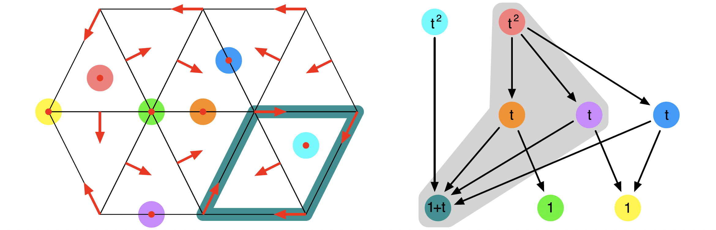
is always an isolated invariant set. Nevertheless, not every isolated invariant set is of this form. For example, the figure contains the multivector field which was discussed in [BKMW20, Figure 3]. While the underlying simplicial complex and the Forman vector field are depicted in the left panel, the associated Conley-Morse graph is shown on the right. For this combinatorial dynamical system, there exists an isolated invariant set which contains only the four Morse sets within the gray region under the graph. More details can be found in A Planar Forman Vector Field.

Morse decompositions and intervals can be easily computed and manipulated in ConleyDynamics.jl using the following commands:

• The function morse_sets expects a Lefschetz complex and a multivector field as arguments, and returns the Morse sets of the finest Morse decomposition as a Vector{Vector{Int}} or Vector{Vector{String}}, matching the format used for the multivector field. If the optional argument poset=true is added, then the function also returns a matrix which encodes the Hasse diagram of the poset $\mathbb{P}$. Note that this is the transitive reduction of the full poset, i.e., it only contains necessary relations.
• The function morse_interval computes the isolated invariant set for a Morse set interval. The three input arguments are the underlying Lefschetz complex, a multivector field, and a collection of Morse sets. The latter should be determined using the function morse_sets. The function returns the smallest isolated invariant set which contains the Morse sets and their connections as a Vector{Int}. The result can be converted to label form using convert_cells.
• The function restrict_dynamics restricts a multivector field to a Lefschetz subcomplex. The function expects three arguments: A Lefschetz complex lc, a multivector field mvf, and a subcomplex of the Lefschetz complex which is given by the locally closed set represented by lcsub. It returns the associated Lefschetz subcomplex lcreduced and the induced multivector field mvfreduced on the subcomplex. The multivectors of the new multivector field are the intersections of the original multivectors and the subcomplex.
• Finally, the function remove_exit_set removes the exit set for a multivector field on a Lefschetz subcomplex. It is assumed that the Lefschetz complex lc is a topological manifold and that mvf contains a multivector field that is created via either create_planar_mvf or create_spatial_mvf. The function identifies cells on the boundary at which the flows exits the region covered by the Lefschetz complex. If this exit set is closed, one has found an isolated invariant set and the function returns a Lefschetz complex lcr restricted to it, as well as the restricted multivector field mvfr. If the exit set is not closed, a warning is displayed and the function returns the restricted Lefschetz complex and multivector field obtained by removing the closure of the exit set. In the latter case, unexpected results might be obtained.

The first two of these functions rely heavily on the Julia package Graphs.jl.

Connection Matrices

While a Morse decomposition represents the basic structure of the global dynamics of a combinatorial dynamical system, it does not directly provide more detailed information about the dynamics between them – except for the poset order on the Morse sets. But which of the associated connecting sets actually have to be nonempty? The algebra behind this question is captured by the connection matrix. The precise notion of connection matrix was introduced in [Fra89], see also [HMS21], as well as the book [MW25] which treats connection matrices specifically in the setting of multivector fields and provides a precise definition of connection matrix equivalence, even across varying posets.

Since the precise definition of a connection matrix is beyond the scope of this manual, we only state what it is as an object, what its main properties are, and how it can be computed in ConleyDynamics.jl. Assume therefore that we are given a Morse decomposition $\mathcal{M}$ of an isolated invariant set $S$. Then the connection matrix is a linear map

\[ \Delta \; : \; \bigoplus_{q \in \mathbb{P}} CH_*(M_q) \to \bigoplus_{p \in \mathbb{P}} CH_*(M_p) ,\]

i.e., it is a linear map which is defined on the direct sum of all Conley indices of the Morse sets in the Morse decomposition. One usually writes the connection matrix $\Delta$ as a matrix in the form $\Delta = (\Delta(p,q))_{p,q \in \mathbb{P}}$, which is indexed by the poset $\mathbb{P}$, and where the entries $\Delta(p,q) : CH_*(M_q) \to CH_*(M_p)$ are linear maps between homological Conley indices. If $I$ denotes an interval in the poset $\mathbb{P}$, then one further defines the restricted connection matrix

\[ \Delta(I) \; = \; \left( \Delta(p,q) \right)_{p,q \in I} \; : \; \bigoplus_{p \in I} CH_*(M_p) \to \bigoplus_{p \in I} CH_*(M_p) .\]

Any connection matrix $\Delta$ has the following fundamental properties:

• The matrix $\Delta$ is strictly upper triangular, i.e., if $\Delta(p,q) \not= 0$ then $p < q$.
• The matrix $\Delta$ is a boundary operator, i.e., we have $\Delta \circ \Delta = 0$, and $\Delta$ maps $k$-th level homology to $(k-1)$-st level homology for all $k \in \mathbb{Z}$.
• For every interval $I$ in $\mathbb{P}$ we have

  \[ H_*\Delta(I) \; = \; \mathrm{ker}\, \Delta(I) / \mathrm{im}\, \Delta(I) \; \cong \; CH_*(M_I) .\]

  In other words, the Conley index of a Morse interval can be determined via the homology of the associated connection matrix minor $\Delta(I)$.
• If $\{ p, q \}$ is an interval in $\mathbb{P}$ and $\Delta(p,q) \neq 0$, then the connection set $\mathcal{C}(M_q,M_p)$ is not empty.

We would like to point out that these properties do not characterize connection matrices. In practice, a given multivector field can have several different connection matrices. These in some sense encode different types of dynamical behavior that can occur in the system. Nonuniqueness, however, cannot be observed if the underlying system is a gradient combinatorial Forman vector field on a Lefschetz complex. These are multivector fields in which every multivector is either a singleton, and therefore a critical cell, or a two-element Forman arrow. In addition, a gradient combinatorial Forman vector field cannot have any nontrivial periodic solutions, i.e., periodic solutions which are not constant and therefore critical cells. For such combinatorial vector fields, the following result was shown in [MW25].

In ConleyDynamics.jl connection matrices can be computed over arbitrary finite fields or the rationals:

• The function connection_matrix computes a connection matrix for the multivector field mvf on the Lefschetz complex lc over the field associated with the Lefschetz complex boundary matrix. The function returns an object of type ConleyMorseCM, which is further described below. If the optional argument returnbasis=true is given, then the function also returns a dictionary which gives the basis for the connection matrix columns in terms of the original cell labels.

At the present time, there are four different algorithms implemented for the computation of connection matrices. A specific algorithm can be selected by passing the optional argument algorithm::String:

• algorithm = "DLMS" selects the original algorithm due to Dey, Lipinski, Mrozek, and Slechta [DLMS24]. This algorithm is based on matrix reductions, and performs a full similarity transformation.
• algorithm = "DHL" selects the more efficient algorithm due to Dey, Haas, and Lipinski [DHL26], which does not perform a complete reduction.
• algorithm = "HMS" selects the algorithm due to Harker, Mischaikow, and Spendlove [HMS21], which is based on discrete Morse theory, i.e., on the use of gradient Forman vector fields to preprocess the underlying Lefschetz complex.
• algorithm = "pmorse" selects a parallelized algorithm based on Morse reductions. For this to take effect, Julia has to be started with multi-threading enabled.

By default, the function connection_matrix uses the parallel Morse reduction algorithm pmorse. However, if the flag returnbasis::Bool=true is given the function has to choose the slower matrix-based one, that is, it automatically uses algorithm = "DLMS". A detailed performance comparison of all four algorithms, including reproducible timing examples, is provided in the section Algorithm Comparisons below.

The connection matrix is returned in an object with the composite data type ConleyMorseCM. Its docstring is as follows:

ConleyMorseCM{T}

To illustrate these fields further, we briefly illustrate them for the example associated with the last figure, see again A Planar Forman Vector Field. For reference, the underlying simplicial complex and Forman vector field are shown in the next figure.

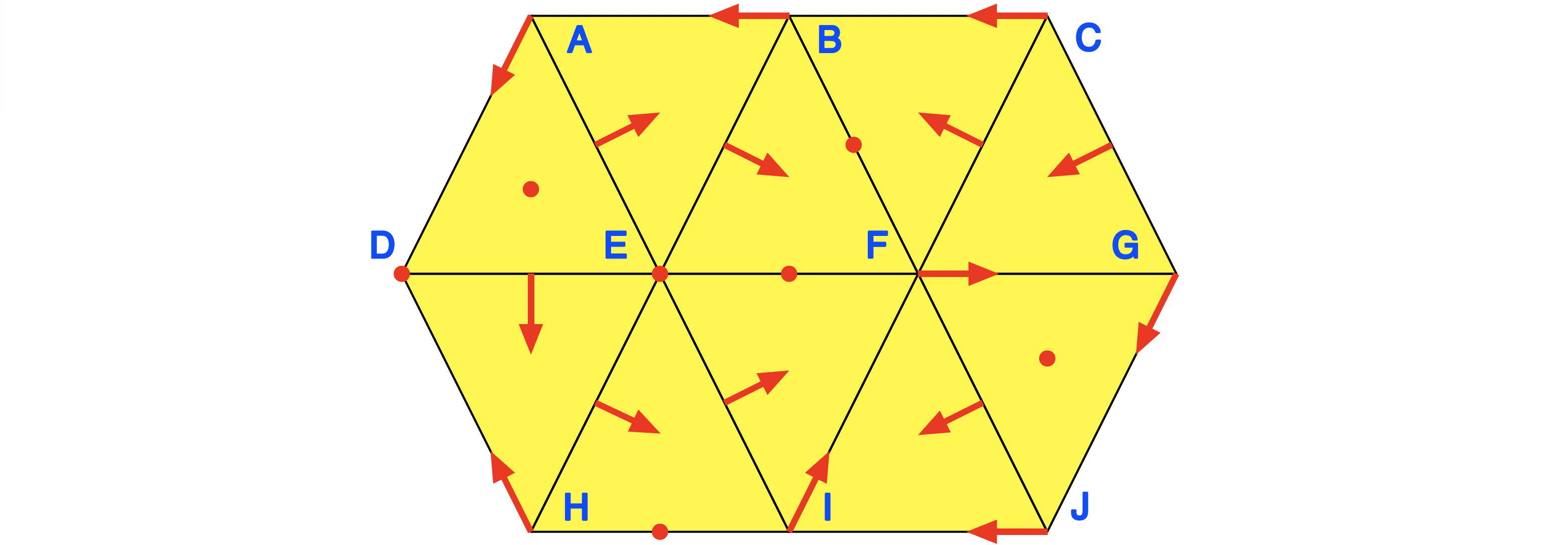
The underlying Lefschetz complex, multivector field, and connection matrix can be computed over the field $GF(2)$ as follows:

lc, mvf = example_forman2d()
cm = connection_matrix(lc, mvf)
sparse_show(cm.matrix)

 . . . . 1 . 1 . .
 . . . . . 1 . . .
 . . . . 1 1 1 . .
 . . . . . . . . 1
 . . . . . . . 1 .
 . . . . . . . . .
 . . . . . . . 1 .
 . . . . . . . . .
 . . . . . . . . .

The field cm.poset indicates which Morse set each column belongs to, while the field cm.labels shows which cell label the column corresponds to. For the example one obtains:

print(cm.poset)

[1, 2, 3, 3, 4, 5, 6, 7, 8]

print(cm.labels)

["D", "E", "I", "FG", "BF", "EF", "HI", "ADE", "FGJ"]

Note that except for the third and fourth column, all columns belong to unique Morse sets whose Conley index is a one-dimensional vector space. The third and fourth column correspond to the periodic orbit, whose Conley index is a two-dimensional vector space. The Conley indices for all eight Morse sets can be seen in the field cm.conley:

cm.conley

8-element Vector{Vector{Int64}}:
 [1, 0, 0]
 [1, 0, 0]
 [1, 1, 0]
 [0, 1, 0]
 [0, 1, 0]
 [0, 1, 0]
 [0, 0, 1]
 [0, 0, 1]

The full associated Morse sets are list in cm.morse:

cm.morse

8-element Vector{Vector{String}}:
 ["D"]
 ["E"]
 ["F", "G", "I", "J", "FG", "FI", "GJ", "IJ"]
 ["BF"]
 ["EF"]
 ["HI"]
 ["ADE"]
 ["FGJ"]

As the final struct field, the entry cm.complex returns the connection matrix as a Lefschetz complex in its own right. This is useful for determining the Conley indices of Morse intervals. In our example, the cells of the new Lefschetz complex are given by

cm.complex.labels

9-element Vector{String}:
 "D"
 "E"
 "I"
 "FG"
 "BF"
 "EF"
 "HI"
 "ADE"
 "FGJ"

The Morse interval consisting of the two index 2 critical cells $\mathbf{ADE}$ and $\mathbf{FGJ}$ should have as Conley index the sum of the two individual indices, and the following computation demonstrates this:

conley_index(cm.complex, ["ADE", "FGJ"])

3-element Vector{Int64}:
 0
 0
 2

In contrast, since there is exactly one connecting orbit between $\mathbf{ADE}$ and $\mathbf{BF}$, the Conley index of this interval should be trivial:

conley_index(cm.complex, ["ADE", "BF"])

3-element Vector{Int64}:
 0
 0
 0

Finally, there are exactly two connecting orbits between the Morse sets $\mathbf{ADE}$ and $\mathbf{EF}$, and therefore the Conley index of this last interval is again the sum of the separate indices:

conley_index(cm.complex, ["ADE", "EF"])

3-element Vector{Int64}:
 0
 1
 1

In order to simplify the inspection of connection matrices, the function sparse_show has a special method for an argument of type ConleyMorseCM. In our example, it produces the following output:

sparse_show(cm)

   ┆   D   E   I  FG  BF  EF  HI ADE FGJ
---┆------------------------------------
  D┆   .   .   .   .   1   .   1   .   .
  E┆   .   .   .   .   .   1   .   .   .
  I┆   .   .   .   .   1   1   1   .   .
 FG┆   .   .   .   .   .   .   .   .   1
 BF┆   .   .   .   .   .   .   .   1   .
 EF┆   .   .   .   .   .   .   .   .   .
 HI┆   .   .   .   .   .   .   .   1   .
ADE┆   .   .   .   .   .   .   .   .   .
FGJ┆   .   .   .   .   .   .   .   .   .

In this way, one can easily see which Morse sets correspond to the columns and rows of the connection matrix.

Algorithm Comparisons

All four algorithms implement the same mathematical task and are guaranteed to return a valid connection matrix for any given input. However, they differ considerably in their underlying approach and their computational behavior as the size of the Lefschetz complex grows. Note that when the connection matrix is not unique, different algorithms may return different — but equally valid — connection matrices.

The matrix-reduction algorithm DLMS works by directly reducing the boundary matrix through column and row operations, while DHL uses only column operations. Their structure is relatively straightforward to follow. The Morse-theory-based algorithms HMS and pmorse first compute a discrete Morse matching to simplify the complex before performing the reduction, which introduces some fixed overhead but can pay off significantly on larger inputs. The parallelized algorithm pmorse additionally distributes parts of the Morse matching computation across multiple threads, and therefore benefits from starting Julia with julia --threads N for some suitable number of threads N.

The following two examples illustrate how the runtime characteristics differ depending on the problem size. The timings were obtained on a standard laptop; exact results will vary by machine, but the relative scaling behavior is representative.

Small Complexes

For a small example one can use the built-in example_forman2d, which creates a Lefschetz complex with 39 cells:

using ConleyDynamics
lc, mvf = example_forman2d()
for alg in ["DLMS", "DHL", "HMS", "pmorse"]
    println(alg, ":  ", @elapsed connection_matrix(lc, mvf, algorithm=alg), " s")
end

Representative timings on this example are as follows:

On small complexes the matrix-reduction algorithms DLMS and DHL perform very efficiently, since the column and row reductions operate on a small matrix. The Morse-based algorithms HMS and pmorse carry a relatively large overhead at this scale from constructing the Morse matching, which does not yet pay off for such small inputs.

Large Complexes

For a more demanding example one can use the planar flow from the section Analysis of a Planar System, with a finer triangulation than used there:

using ConleyDynamics, Random
Random.seed!(1234)
function planarvf(x::Vector{Float64})
    x1, x2 = x
    y1 = x1 * (1.0 - x1*x1 - 3.0*x2*x2)
    y2 = x2 * (1.0 - 3.0*x1*x1 - x2*x2)
    return [y1, y2]
end
lc  = create_simplicial_delaunay(400, 400, 3, 50, euclidean=true)
lc  = rescale_coords(lc, -1.2, 1.2)
mvf = create_planar_mvf(lc, planarvf)
println("ncells = ", lc.ncells)
for alg in ["DLMS", "DHL", "HMS", "pmorse"]
    println(alg, ":  ", @elapsed connection_matrix(lc, mvf, algorithm=alg), " s")
end

This creates a Lefschetz complex with approximately 71,000 cells. Representative timings on this example, using four threads for pmorse, are as follows:

At this scale the picture changes substantially. The Morse-theory-based algorithms scale considerably more favorably than the matrix-reduction approaches. Among the matrix-based algorithms, DHL — due to Dey, Haas, and Lipinski — is significantly more efficient than DLMS, which performs a complete similarity transformation of the matrix. The algorithm HMS due to Harker, Mischaikow, and Spendlove, which preprocesses the complex using discrete Morse theory, requires much less time at this scale. The parallel algorithm pmorse achieves a further reduction in wall-clock time when multiple threads are available.

The algorithm DLMS is the only one that supports the optional flag returnbasis=true, which returns the basis of each connection matrix column in terms of the original cell labels. When this flag is passed to connection_matrix, the function automatically selects DLMS regardless of the algorithm keyword.

Forman's Morse Complex

The package ConleyDynamics.jl also provides some support for studying Forman gradient vector fields directly, using the notions introduced in [For98b]. In this paper, Forman used the concept of a combinatorial flow $\Phi$ to study the forward orbits generated by the Forman vector field. The map $\Phi$ is a chain map which is chain homotopic to the identity, and it therefore mimics the concept of a time-1-map associated with a dynamical system. Forman shows that upon iteration this map stabilizes as a map $\Phi^\infty$, which encodes the connecting orbits in the associated combinatorial dynamical system. This stabilized combinatorial flow can then be used to find the connection matrix in this case. For more details, we refer to [MW25, Chapter 8]. The combinatorial flow and its stabilized version can be computed using the following two functions.

• forman_comb_flow expects a Lefschetz complex and a Forman vector field as input arguments. It returns matrix representations of Forman's combinatorial flow $\Phi$, as well as of the associated chain homotopy $\Gamma$ between the flow chain map and the identity.
• forman_stab_flow also requires both a Lefschetz complex and a Forman vector field as arguments. It then returns matrix representations of Forman's stabilized combinatorial flow $\Phi^\infty$, and of the associated chain homotopy $\Gamma^\infty$. This time, there is a third return argument stabilized. This boolean flag indicates whether or not the combinatorial flow stabilized. If it did not, then the returned chain map is the last computed iterate, together with the corresponding chain homotopy. There are two possible reasons for failing stabilization: Either the underlying Forman vector field is not gradient (note that this is not checked!), or the maximal number of iterations has been reached. In the latter case, one just has to pass the optional paramter maxit with a larger number of allowed iterations.
• forman_conley_maps computes the chain maps and chain homotopies associated with the Conley complex of a Forman gradient vector field. The function expects a Lefschetz complex and a Forman gradient vector field as arguments, and it returns:
  • pp:SparseMatrix: The chain equivalence which maps the Lefschetz complex to the Conley complex.
  • jj:SparseMatrix: The chain equivalence which maps the Conley complex to the Lefschetz complex.
  • hh:SparseMatrix: The chain homotopy between jj*pp and the identity map on the Lefschetz complex.
  • cc:Cells: The list of critical cells of the Forman vector field which make up the Conley complex.
  These quantities are computed using Forman's stabilized combinatorial flow.
• forman_gpaths can be used to find gradient paths in a Forman gradient vector field. There are two methods for this function, which are accessible via multiple dispatch as follows.
  • The call forman_gpaths(lc, fvf, x) determines all maximal gradient paths of the Forman gradient field fvf on the Lefschetz complex lc starting at x. These are solution paths which consist exclusively of Forman vectors, i.e., they contain an even number of cells whose dimensions alternate between $\dim x$ and $1 + \dim x$. Every cell of dimension $\dim x$ is an arrow source which is followed by its arrow target, while every cell of dimension $1 + \dim x$ is an arrow target which is succeeded by a cell in its boundary, and which in turn is the source of a different arrow, as long as such a cell exists.
  • The call forman_gpaths(lc, fvf, x, y) computes all Forman gradient paths between the cells x and y. Nontrivial paths are only returned if $|\dim x - \dim y| \le 1$. More precisely, the following paths are returned:
    • If $\dim x = \dim y - 1$, the function returns all solution paths between x and y which consist entirely of Forman arrows. All the sources have the dimension of x, and the targets the dimension of y.
    • For $\dim x = \dim y$ the function finds all solution paths p between x and y for which p[1:end-1] is a Forman gradient path in the above sense, and p[end] lies in the boundary of p[end-1] and is different from the cell p[end-2]. For this, the length of the path has to be at least 3. If on the other hand one has $x = y$, then only a 1-element path is returned.
    • Finally, if $\dim x = \dim y + 1$, then the function returns all solution paths p between x and y for which p[2:end] is a Forman gradient path in the sense of the second item, and p[2] lies in the boundary of p[1].
    In all other cases an empty collection is returned.
• forman_path_weight expects the arguments lc:LefschetzComplex and path::Cell and computes the weight of the Forman gradient path path in the Lefschetz complex lc. It is expected that the dimensions of the first and the last cell in the path differ by at most 1. In case they have equal dimension, and the path has length larger than 1, the first cell has to be an arrow source. This function also has a second method associated with its name, in which the second argument is of type CellSubsets, i.e., it contains a collection of Forman gradient paths. In the case, the function returns the sum of all weights of these paths.

The following two functions allow one to extract cells of certain types from a Forman vector field:

• forman_critical_cells extracts all critical cells from a Forman vector field.
• forman_all_cell_types returns lists of cells of all three types in a Forman vector field. More precisely, it returns vectors which contain the critical cells, the arrow sources, and the arrow targets.

For analyzing or applying Forman's combinatorial flow, one needs to work with sparse vector representations of chains. These are elements of the chain groups of the underlying Lefschetz complex, which are then represented as sparse matrices consisting of exactly one column. In this form, they can be multiplied by the matrix of the combinatorial flow, which in turn determines the image of the chain under the flow. In general, these vectors are extremely sparse, and only contain a handfull of nonzero entries. ConleyDynamics.jl therefore provides the following two functions for the creation and analysis of sparse chain vectors:

• chain_vector is a function that simplifies the creation of a sparse vector representation of a chain. The chain can be specified by simply listing the cells in the support of the chain. If no coefficients are specified, then the chain is just the sum of these cells, each with coefficient 1. The function has several associated methods: The coefficients of the chain can be omitted or specified, and the cells can be listed in index or label form. More details can be found in the description of each method.
• chain_support extracts the support of a chain given as a sparse vector. In its simplest form, the function returns a Vector{String} which contains the labels of all the cells which have nonzero coefficients in the chain. If one passes the optional parameter coeff=true, then the function returns two arguments: In addition to the vector of labels as above, it also returns the vector of associated coefficients.

References

See the full bibliography for a complete list of references cited throughout this documentation. This section cites the following references: